Spectroscopy is of a foundational importance to physical chemistry, and has been a central fixture in both my own graduate and undergraduate work. In this post I would like to delineate how the birth of spectroscopy stemmed from the study of the solar spectrum, and how sunlight will form the basis of a better global energy conversion system.
Up until widespread electrification of lighting (less than 200 years ago), daylight was the primary light source (not counting gas lamps, candles, fires, and so on). Daylight is sunlight filtered through the atmosphere.1 If, for the sake of example, we consider the atmosphere to be constant (which it most definitely is not, or see why star’s twinkle), then daylight is simply a function of the Sun’s spectrum attenuated by that constant.
The scientific study of sunlight began only 200 years ago (more on that below), but the question of the Sun’s distance to us, its size and age has probably enagaged all civilizations.
The realisation that the Sun must be very far away was made already in antiquity, most notably by the Hellenic astronomer Posidonius the Syrian who in 90 BC calculated the distance and was only wrong by less than half [1]. The Sun’s mechanism and age,2 however, were not correctly determined until the 20th century and the advent of the field of stellar nucleosynthesis. So in a sense, despite living under the same Sun as all our ancestors back to the beginning of humanity, humans have not been in the privileged position of knowing what stuff a star is made of until quite recently (more recent than the invention of the bike, for comparison).
The beginnings of the science of spectroscopy
The observations of “lines” in sunlight, candle-light and electric light seen through single prisms by Wollaston in 1802 [2] can, with hindsight, be considered the beginning of spectroscopy as we know it. But his results might well have been forgotten if Fraunhofer had not made new observations on sunlight 13 years later by adding a telescope to the prism and slit, observing “almost innumerable strong and weak vertical lines which however are darker than the other part of the coloured image; some seem to be almost completely black”3.
![This copper-etching was made by Fraunhofer himself. It shows the full visible spectrum including the famous Fraunhofer lines[^4], some of them named with letters. Above it is the curve of spectral response of the eye to daylight illumination. [Wikimedia, CC-BY-SA](https://commons.wikimedia.org/wiki/File:Fraunhofer_Spektrum_Medium.jpg).](assets/Fraunhofer_Spektrum_Medium.jpg)
Figure 1: This copper-etching was made by Fraunhofer himself. It shows the full visible spectrum including the famous Fraunhofer lines4, some of them named with letters. Above it is the curve of spectral response of the eye to daylight illumination. Wikimedia, CC-BY-SA.
Thanks to Kirchhoff and Bunsen (1859) the relationship5 between dark and bright lines of the same wavelength (absorption vs emission, in modern terms) were understood, and also the unique correspondence of line wavelength to chemical element, thus making the spectrum a fixed frame of reference and seeding the ground for the budding field of astrophysics, a field which bloomed after the Doppler effect was described in 1842.
A few decades later Anders J. Ångström made an important contribution to spectroscopy by mapping one thousand absorption lines in the solar spectrum (and was the first to label the spectrum in units of 10-10 m, later named after him) [3] which was improved on by Rowland who carefully measured 21 thousand lines in 1897. Modern measurements of the solar spectrum have shown that at least 62 elements are certainly present in the Sun’s atmosphere. Considering that by mass 98.4 % of the sun consists of just hydrogen and helium,6 that’s a large variation of heavier elements.
These discoveries all concerned the visible part of the spectrum. But after the development of the optical prism (by the 19th century) scientists began to expand the spectrum beyond visible light: Herschel discovered the infrared part of the solar spectrum in 1800, and Ritter discovered the ultraviolet one a year later. Both spectral regions were found to contain more absorption lines.
The method of detecting and recording one’s observed spectrum improved over the years and was tightly interwoven with the development of photography.
Today we have the line spectra of all naturally occuring elements available
at our fingertips from a variety of tools, here for example the LaTeX pgf-spectra
package [5] which builds on spectral data from NIST:
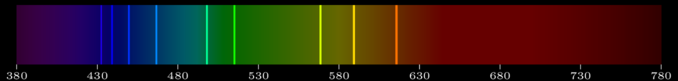
Figure 2: Emission lines of sodium in the visible spectrum.
Sunlight above and below the atmosphere
Whereas the spectral composition of daylight varies dramatically with season, location and time of day, the amount of sunlight that reaches the top of Earth’s atmosphere (i.e., the total solar irradiance, TSI, previously known as the solar constant) has been experimentally shown to be practically constant over time, and any variations are certainly not enough to account for the rise in mean global surface temperature observed since the industrial revolution.
The first experimental observations in the modern sense of the solar constant (i.e., TSI) were made in the early 19th century by Herschel and Poillet using their newly invented actinometer and pyrheliometer, respectively. They were soon followed by John Ericsson, who invented what he called a “solar calorimeter” that improved on the earlier devices by taking the atmospheric column above the measurement into better account and arrived at a value of 7.11 BTU7 per minute per square foot of surface at the boundary of the atmosphere [6], which is equivalent to \(\SI{1332}{\watt\per\square\metre}\) and very close to the modern value.

Figure 3: Solar irradiation at the top of the atmosphere (AM0, yellow area) and at sea level (AM1.5G, red area), as well as the solar irradiance modelled as a black body (black curve). Also shown is the total irradiance for each of the UV, Vis, and NIR spectral regions for the AM0 and AM1.5G spectra.
Since 1978, solar irradiance above the Earth’s atmosphere is continuously measured by satellite-based radiometers, which is then averaged over the year and corrected to a distance of exactly 1 AU to yield the TSI. Indeed, one of the reasons the “solar constant” was renamed to TSI is that it is not really constant, but changes depending on solar output, which varies mainly with the solar sunspot cycle (which goes from minimum to maximum magnetic activity in 11-year cycles). The last solar minimum was in 2022, and TSI during the preceding minimum in 2011 was \(\SI{1360.8\pm0.5}{\watt\per\square\metre}\) [7]. But note that whereas the solar irradiance at the top of Earth’s atmosphere varies quite a lot depending on several periodic phenonema of varying timescales, TSI varies very little. For example, TSI shows less than 0.2 % variation due to the sunspot cycle [8].
Below the atmosphere, that is, on the ground we (that is, in the photovoltaic field) almost always resort to the ASTM G173-03 solar reference spectra, which give us a full solar spectrum (250 nm–4000 nm) depending primarily on the air mass, which is a convenient way to express latitude. Of course, more detailed models exist, but for the purpose of scientific reports such international standards are really all that is needed.
Notes and links
If you are interested in the physics of daylight and the history of its study I can recommend the treatise by Henderson [1] (a book which might be hard to find, though).
- Spectroscopy, Britannica. A remarkably comprehensive article.
- What is the Mössbauer effect?, Skulls in the Stars (2023). Great explainer of absorption/emission in atoms.
- Invisible light: prism experiments through the centuries, Wallifaction (2014)
- A brief (incomplete) history of light and spectra
- Electrification, Wikipedia
- The historical cost of light
- Introduction to spectroscopy, NASA
- UV-visible spectroscopy, LibreTexts Chemistry
- Actinometer, Wikipedia
- Pyrheliometer, Wikipedia
- Ångström, Wikipedia
- Spectroscopy, Wikipedia
- History of spectroscopy, Wikipedia
- Air mass (solar energy), Wikipedia
- Spectrometer, spectroscope, and spectrograph, excerpt from Field Guide to Spectroscopy [9]
- Spectrophotometry, Wikipedia
- Spectrophotometry, LibreTexts Chemistry
- Atomic spectroscopic data, NIST
- Total solar irradiance data, Laboratory for Atmospheric and Space Physics, University of Colorado Boulder (2020)
- Using spectroscopy for solar irradiance and UV measurements, AZO Materials (2017)
- Solar irradiance, ed. Rob Garner, NASA (2017)
- Solar radiation measurements, presentation slides (PDF) from workshop for the National Association of State Universities and Land Grant Colleges, Tom Stoffel and Steve Wilcox, NREL (2004)
- Enhancements enable solar simulators to shed light on new photovoltaic designs, Jay Jeong (2007)
- What is an optical spectrometer?, West and Harrell, Oxford Instruments (2022)
Session info
## Linux 5.15.0-78-generic #85-Ubuntu SMP Fri Jul 7 15:25:09 UTC 2023 x86_64## R version 4.1.3 (2022-03-10)
## Platform: x86_64-pc-linux-gnu (64-bit)
## Running under: Ubuntu 22.04.3 LTS
##
## Matrix products: default
## BLAS: /usr/lib/x86_64-linux-gnu/blas/libblas.so.3.10.0
## LAPACK: /usr/lib/x86_64-linux-gnu/lapack/liblapack.so.3.10.0
##
## locale:
## [1] LC_CTYPE=en_US.UTF-8 LC_NUMERIC=C
## [3] LC_TIME=sv_SE.UTF-8 LC_COLLATE=en_US.UTF-8
## [5] LC_MONETARY=en_US.UTF-8 LC_MESSAGES=en_US.UTF-8
## [7] LC_PAPER=en_US.UTF-8 LC_NAME=C
## [9] LC_ADDRESS=C LC_TELEPHONE=C
## [11] LC_MEASUREMENT=en_US.UTF-8 LC_IDENTIFICATION=C
##
## attached base packages:
## [1] stats graphics grDevices utils datasets methods base
##
## other attached packages:
## [1] bandgaps_0.1.1.9000 photoec_0.4.2.9000 common_0.1.2 stringr_1.4.0
## [5] dplyr_1.0.10 tibble_3.1.8 tidyr_1.2.1 ggplot2_3.3.6
## [9] knitr_1.39 git2r_0.30.1 here_1.0.1 conflicted_1.1.0
##
## loaded via a namespace (and not attached):
## [1] tidyselect_1.2.0 xfun_0.31 bslib_0.4.0 purrr_0.3.5
## [5] colorspace_2.0-3 vctrs_0.5.1 generics_0.1.3 htmltools_0.5.3
## [9] yaml_2.3.5 utf8_1.2.2 rlang_1.0.6 jquerylib_0.1.4
## [13] pillar_1.8.1 glue_1.6.2 withr_2.5.0 DBI_1.1.3
## [17] lifecycle_1.0.3 munsell_0.5.0 blogdown_1.10 gtable_0.3.0
## [21] memoise_2.0.1 evaluate_0.15 labeling_0.4.2 fastmap_1.1.0
## [25] fansi_1.0.3 highr_0.9 scales_1.2.0 cachem_1.0.6
## [29] jsonlite_1.8.0 farver_2.1.1 digest_0.6.29 stringi_1.7.8
## [33] bookdown_0.27 grid_4.1.3 rprojroot_2.0.3 cli_3.4.1
## [37] tools_4.1.3 magrittr_2.0.3 sass_0.4.2 crayon_1.5.1
## [41] pkgconfig_2.0.3 ellipsis_0.3.2 assertthat_0.2.1 rmarkdown_2.16
## [45] R6_2.5.1 compiler_4.1.3## Commit: ec42cbcbc2cd1968feedcfe4b13f4f15d76c32e9
## Author: taha@luxor <taha@chepec.se>
## When: 2023-10-09 20:58:44 GMT
##
## Added a link.
##
## 1 file changed, 2 insertions, 1 deletions
## index.Rmd | -1 +2 in 1 hunk## working directory cleanReferences
In the UV to NIR spectral range the atmosphere can be considered a combination of multiple band-stop filters, where different compounds block specific wavelengths (see atmospheric window).↩︎
The realisation that the Sun must be very far away from us was much easier to grasp than the mechanism that powered it, and by extension, its age. Famously, even Lord Kelvin held firm to the view that the Sun was at most a few hundred million years old, despite many of his contemporaries arguing that it was necessarily much older (in fairness, fusion was unknown at the time).↩︎
The quote is from [1, p. 9]. Wollaston’s paper (in the original German) can be read at the Internet Archive. For a more accessible source, see the notes in the Wikipedia article.↩︎
Fraunhofer lines, i.e., the black spectral lines seen when sunlight is split in a spectrometer, formed due to absorption by various atom species in the gaseous state in the Sun’s atmosphere.↩︎
Stokes independently discovered this principle but never claimed any credit [1]. And Foucault had observed both emission and absorption lines of sodium in a flame (the latter by placing a bright arc behind the flame) but never pursued the subject further.↩︎
This was only realised in 1925 by Cecilia Payne-Gaposchkin in her doctoral thesis, which primarily dealt with how the large variations in absorption line strength (from star to star) in stellar spectra was due to differing temperatures and not chemical composition [4]. Incidentally, her data also demonstrated a clear abundance of hydrogen and helium in the sun, but she did not quite believe her own analysis on that point, writing “the enormous abundance derived for these elements in the stellar atmosphere is almost certainly not real”.↩︎
BTU, British thermal unit, is a non-SI unit that is no longer used in science but still finds use in the fossil fuel sector. Converting from it to kWh is not straightforward (depends on whether the kWh was produced from combustible or non-combustible generation method). The International Energy Agency recently updated its recommended conversion factor. ↩︎