In this post we share some experimentally recorded UV-Vis-NIR spectra and absorption coefficient1 curves of the dyes eriochrome black T (EBT), methylene blue (MB), methyl orange (MO), and reactive black 5 (RB5) in aqueous solution. For EBT, MB and MO we also report the absorption coefficient in the presence of 10% EtOH (by volume).
This post also includes a small study on pH and conductivity at room temperature of the same dyes.
This post is likely of interest for research into photocatalytic dye degradation, and the dataset is shared in this blog post’s repo on Codeberg (as R dataset files).
Spectral absorption coefficients
To make the absorption coefficient curves (figure 2) less noisy, we will start by calculating the average absorbance value inside a wavelength band \(\SI{10}{\nm}\) wide centered on the main absorbance band of each dye. This band is shown as a shaded yellow area in figure 1 below.
Unfortunately, I’ve lost the original data for RB5 in water, but we still have the plot of those measurements, which is shown as an inset. However, the shape of the absorption coefficient curve of RB5 in only water can be assumed to very closely follow that of the dye in the presence of alcohol (figure 1).

Figure 1: UV-Vis spectra of EBT, MB, MO, and RB5 at varying concentrations in aqueous solution with or without the addition of a small amount of alcohol.
EBT is the only dye that shows isosbestic points between the spectra of the different solvents. With the exception of MB, the other dyes show only a slight overall intensity decrease when introducing alcohol into the solvent. MB demonstrates a very obvious, yet subtle, intensity change in its main shoulder when adding EtOH to the solvent, which I have discussed my paper [1].
EBT is also the only dye (of the four tested) that shows spectral changes dependent on concentration, which indicates formation of new molecular species at higher concentrations. In contrast, the other dyes are all well-behaved as the concentration changes, in the sense that the position and shape of their peaks are independent of concentration, which indicates that the dye solution contains the same molecular components irrespective of concentration (within the studied range).
From the absorption spectra of a series of concentrations and by applying the Beer-Lambert law we can calculate the absorption coefficients for the measured wavelength range.
\[\begin{equation} A = \epsilon lc \;\Longleftrightarrow\; \epsilon = \frac{A}{lc} \end{equation}\]
Given that absorbance is unit-less, and with \([l]=\si{\cm}\) and \([c]=\si{\mol\per\litre}\), then the unit of the molar absorption coefficient is \([\epsilon]=\si{\litre\per\mole\per\cm}\) which is how it is usually given.
We will calculate the absorption coefficient \(\epsilon\) for each wavelength step, by dye and solvent.Effectively we are calculating one linear fit (abs vs conc) for each wavelength step.
# this chunk calculates linear fits for every single wavelength step, which is time-consuming
if (file.exists(here::here("assets/abscoeff.rda"))) {
   abs.coeff <- LoadRData2Variable(here::here("assets/abscoeff.rda"))
} else {
   # replace both MeOH and EtOH strings with the more generic ROH for easier looping
   df.dye %<>%
      mutate(solution = ifelse(solution == "H2O+MeOH", "H2O+ROH", solution)) %>%
      mutate(solution = ifelse(solution == "H2O+EtOH", "H2O+ROH", solution))
   # convert df.dye$conc from factor to numeric
   df.dye$conc <-
      df.dye$conc %>% as.character() %>% as.numeric()
   # loop over each spectra by dye and solution
   dyes      <- unique(df.dye$dye)
   solutions <- unique(df.dye$solution)
   wl.steps  <- unique(df.dye$wavelength)
   # hold the results of the looping in a new dataframe
   abs.coeff <-
      data.frame(
         wavelength = rep(wl.steps, length(dyes) * length(solutions)),
         dye = "",
         solution = "",
         k = NA,
         m = NA,
         rsq = NA,
         adj.rsq = NA,
         concentrations = "") # uM
   i <- 0
   # NOTE: this loop is time-consuming, so I've intentionally made it chatty
   for (d in 1:length(dyes)) {
      message("Dye: ", dyes[d])
      if (dyes[d] == "RB5") {
         # we only have H2O+ROH spectrum for RB5, so we need to reset solutions so the next inner loop doesn't    fail
         solutions <- "H2O+ROH"
      }
      for (s in 1:length(solutions)) {
         message("Dye: ", dyes[d], " :: Solution: ", solutions[s])
         # varying conc of a particular dye and solution
         for (w in 1:length(wl.steps)) {
            # to keep track of the current row in abs.coeff, we will use a counter var
            i <- i + 1
            message("[", i, "] ", dyes[d], " :: ", solutions[s], " :: ", wl.steps[w], " nm")
            # temporary dataframe which we will use to calculate linear fits (abs coeff) for each wl step
            intensity.by.wl <-
               df.dye %>%
               filter(dye == dyes[d]) %>%
               filter(solution == solutions[s]) %>%
               filter(wavelength == wl.steps[w]) %>%
               select(sampleid, wavelength, intensity, conc, dye, solution)
            # now we can calculate abs coeff for this solution and dye at the current wavelength
            this.fit <- lm(data = intensity.by.wl, formula = intensity ~ conc)
            # save the concentrations for reference
            abs.coeff$concentrations[i] <-
               paste(sort(intensity.by.wl$conc), collapse = ", ")
            # save R-squared and adjusted R-squared
            abs.coeff$rsq[i] <- summary(this.fit)$r.squared
            abs.coeff$adj.rsq[i] <- summary(this.fit)$adj.r.squared
            # save coefficients of linear fit
            abs.coeff$m[i] <- this.fit$coefficients[1]
            abs.coeff$k[i] <- this.fit$coefficients[2]
            # solution and dye
            abs.coeff$solution[i] <- unique(intensity.by.wl$solution)
            abs.coeff$dye[i] <- unique(intensity.by.wl$dye)
         }
      }
   }
   # adjust units of abs coeffs to L mol-1 cm-1 (from L umol-1 cm-1)
   abs.coeff$k <- 1E6 * abs.coeff$k
   abs.coeff$m <- 1E6 * abs.coeff$m
   # and last, because we are missing H2O-only spectrum for RB5, remove the empty rows in abs.coeff
   # (faster to clean-up in this way than to rewrite this entire loop)
   abs.coeff <- abs.coeff %>% filter(!is.na(k))
   # save abs.coeff
   save(abs.coeff, file = here::here("assets/abscoeff.rda"))
}
Figure 2: Spectral absorption coefficients in aqueous solution for Eriochrome Black T, methylene blue, methyl orange, and reactive black 5, as calculated from the absorbance–concentration series shown in figure 1.
Experimental notes
Preparation of dye stock solutions

Figure 3: Chemical structures of the dyes, as commonly given.
Weighed up EBT and MB powder. Used a Mettler AT261 DeltaRange balance at the XPS room (Ångström bldg 3, level 3). The balance has a readability of \(\SI{0.01}{\mg}\) (cf. the balance’s technical specs), but to make use of it the operator has to press a button (otherwise you get the lower, but still respectable, \(\SI{0.1}{\mg}\) readibility), but I only realised this after I had weighed the EBT powder. But at least the MB measurement used the full sensitivity range of the balance.
Measured weight of EBT was \(\SI{46.3}{\mg}\) (error with respect to calculated weight +0.35%). Measured weight of MB was \(\SI{32.01}{\mg}\) (error with respect to calculated weight +0.08%). Measured weight of MO was \(\SI{32.84}{\mg}\) (error with respect to calculated weight +0.33%)
All measurements were done using disposable polysterene weighing boats. The MB powder showed some static charge, so I used an anti-static gun on a weighing boat which decreased the “jumpiness” of the particles.
The EBT was likely stored a long time, but the MB and MO were from new, sealed containers.
Both EBT and MB were easily dissolved in water. EBT caused a lot of air bubbles at the solution-air interface at the highest concentrations. MO required ultra-sonication for \(\SI{10}{\minute}\) to dissolve all particles.
Mixing alcohol into the aqueous dye solutions
For EBT and MB, added ca \(\SI{2}{\milli\liter}\) of dye solution using disposable plastic pipette, then added \(\SI{200}{\micro\liter}\) of EtOH with autopipette and agitated the solution until completely mixed.
For MO, added precisely \(\SI{1.8}{\milli\liter}\) of dye solution using an electronic auto-pipette, then added \(\SI{200}{\micro\liter}\) of EtOH with auto-pipette and mixed the solution.
For RB5, added ca \(\SI{2}{\milli\liter}\) of dye solution using disposable plastic pipette, then added \(\SI{200}{\micro\liter}\) of MeOH with auto-pipette and mixed the solution.
In all cases, the mixing was done directly in PMMA macro cuvettes (\(SI{1}{\cm}\) path length).
Configuration of the light-source and spectrometer
Spectrophotometer: OceanOptics HR2000 spectrometer. Light source with both deuterium and halogen lamps. Light transmitted from lamp to cuvette and from cuvette to spectrometer using OceanOptics UV-Vis fibre-optic cables.
For all experiments reported here we used both the deuterium and tungsten lamps of the OOHR2000 spectrometer, giving us an effective wavelength range approximately \(\SIrange{260}{1000}{\nm}\) (the spectrum of this light is shown below).

Figure 4: Spectrum of deuterium (contributes UV) and tungsten (Vis) lamp measured after transmission through approximately of fibre-optic cable and a decimetre of air. The sharp dip at \(\SI{950}{\nm}\) is caused by absorption in the fibre-optic cable.
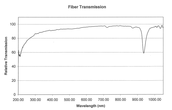
Figure 5: UV-Vis transmittance spectrum of our fibre-optic cable, from calibration experiments courtesy of OceanOptics.
Small study into the pH and conductivity of aqueous dye solutions
I measured pH and conductivity simultaneously for all dye stock solutions, after allowing the solutions to equilibrate with air for at least two hours. The pH and conductivity measurements were done using a handheld Mettler Toledo SevenGo Duo pro™ SG78 pH/ion/conductivity meter.
| sampleid | solute | C/µM | V/mL | pH | T(pH)/°C | σ/(µS/cm) | T(σ)/°C |
|---|---|---|---|---|---|---|---|
| H01AA | EBT | 100.0 | 1000 | 5.881 | 19.0 | 34.60 | 19.1 |
| H01AB | EBT | 50.0 | 500 | 5.908 | 19.1 | 18.56 | 19.4 |
| H01AC | EBT | 20.0 | 250 | 5.901 | 19.0 | 9.37 | 19.3 |
| H01AD | EBT | 10.0 | 500 | 6.254 | 18.9 | 6.17 | 18.9 |
| H01AE | EBT | 5.0 | 200 | 6.096 | 19.0 | 5.34 | 19.2 |
| H01AF | EBT | 2.0 | 250 | 6.169 | 18.9 | 3.44 | 19.2 |
| H02AA | MB | 100.0 | 1000 | 5.993 | 18.7 | 10.12 | 19.2 |
| H02AB | MB | 50.0 | 500 | 5.847 | 18.9 | 7.31 | 19.0 |
| H02AC | MB | 20.0 | 250 | 6.078 | 19.1 | 4.52 | 19.2 |
| H02AD | MB | 10.0 | 500 | 5.938 | 18.9 | 3.67 | 19.0 |
| H02AE | MB | 5.0 | 200 | 5.866 | 18.9 | 3.08 | 19.0 |
| H02AF | MB | 2.0 | 250 | 5.812 | 18.9 | 2.46 | 19.3 |
| H02AG | MB | 1.0 | 250 | 5.964 | 18.7 | 1.72 | 19.4 |
| H02AH | MB | 0.5 | 200 | 6.145 | 18.9 | 1.86 | 19.0 |
| H03AA | MO | 100.0 | 1000 | NA | NA | 10.45 | 22.0 |
| H03AB | MO | 50.0 | 500 | NA | NA | 6.99 | 22.2 |
| H03AC | MO | 20.0 | 250 | NA | NA | 4.49 | 22.3 |
| H03AD | MO | 10.0 | 500 | NA | NA | 4.53 | 22.1 |
| H03AE | MO | 5.0 | 200 | NA | NA | 4.63 | 21.7 |
| H03AF | MO | 2.0 | 250 | NA | NA | 3.22 | 22.7 |
The measured pH of deionised (DI) water at the same experimental conditions was \(\num{6.024}\) and its conductivity was \(\SI{2.35}{\micro\siemens\per\cm}\). Deionised water in contact with air will eventually reach an equilibrium pH 5.7 (the time it takes to reach equilibrium depends on the volume, the shape of the vessel, stirring or not, etc., but is generally on the order of a few hours).
The observed pH values for the different solute concentrations hints at a markedly different acid-base chemistry for EBT and MB, respectively. The following plot shows the change in electrolytic conductivity with concentration for EBT, MB, and MO (the dashed line is the measured pH of DI water, which for the purposes of this visualisation lacks a defined concentration):

Links and notes
- Isosbestic point, Wikipedia
- Equilibrium pH of deionised water in contact with air, Chemistry SE
- pH and composition of carbonic acid solutions, Wikipedia
- Difference between distilled and deionised water, ResearchGate
- Methylene blue, NIH
- Electrolytic conductivity, Wikipedia
Session info
## Linux 5.15.0-78-generic #85-Ubuntu SMP Fri Jul 7 15:25:09 UTC 2023 x86_64## R version 4.1.3 (2022-03-10)
## Platform: x86_64-pc-linux-gnu (64-bit)
## Running under: Ubuntu 22.04.3 LTS
##
## Matrix products: default
## BLAS: /usr/lib/x86_64-linux-gnu/blas/libblas.so.3.10.0
## LAPACK: /usr/lib/x86_64-linux-gnu/lapack/liblapack.so.3.10.0
##
## locale:
## [1] LC_CTYPE=en_US.UTF-8 LC_NUMERIC=C
## [3] LC_TIME=sv_SE.UTF-8 LC_COLLATE=en_US.UTF-8
## [5] LC_MONETARY=en_US.UTF-8 LC_MESSAGES=en_US.UTF-8
## [7] LC_PAPER=en_US.UTF-8 LC_NAME=C
## [9] LC_ADDRESS=C LC_TELEPHONE=C
## [11] LC_MEASUREMENT=en_US.UTF-8 LC_IDENTIFICATION=C
##
## attached base packages:
## [1] stats graphics grDevices utils datasets methods base
##
## other attached packages:
## [1] oceanoptics_0.0.0.9004 common_0.1.2 here_1.0.1
## [4] ggrepel_0.9.1 magick_2.7.3 cowplot_1.1.1
## [7] ggplot2_3.3.6 knitr_1.39 dplyr_1.0.10
## [10] git2r_0.30.1 conflicted_1.1.0
##
## loaded via a namespace (and not attached):
## [1] Rcpp_1.0.9 highr_0.9 bslib_0.4.0 compiler_4.1.3
## [5] pillar_1.8.1 jquerylib_0.1.4 tools_4.1.3 digest_0.6.29
## [9] jsonlite_1.8.0 evaluate_0.15 memoise_2.0.1 lifecycle_1.0.3
## [13] tibble_3.1.8 gtable_0.3.0 pkgconfig_2.0.3 rlang_1.0.6
## [17] cli_3.4.1 DBI_1.1.3 yaml_2.3.5 blogdown_1.10
## [21] xfun_0.31 fastmap_1.1.0 withr_2.5.0 stringr_1.4.0
## [25] generics_0.1.3 vctrs_0.5.1 sass_0.4.2 rprojroot_2.0.3
## [29] grid_4.1.3 tidyselect_1.2.0 glue_1.6.2 R6_2.5.1
## [33] fansi_1.0.3 rmarkdown_2.16 bookdown_0.27 farver_2.1.1
## [37] magrittr_2.0.3 scales_1.2.0 htmltools_0.5.3 assertthat_0.2.1
## [41] colorspace_2.0-3 labeling_0.4.2 utf8_1.2.2 stringi_1.7.8
## [45] munsell_0.5.0 cachem_1.0.6 crayon_1.5.1## Commit: 5ea2dc4e89159b2773568a88901ec0310004dd71
## Author: taha@luxor <taha@chepec.se>
## When: 2023-10-14 19:08:20 GMT
##
## Published!
##
## 10 files changed, 782 insertions, 8 deletions
## README | -8 + 0 in 1 hunk
## assets/EBT.rda | -0 + 0 in 0 hunk (binary file)
## assets/MB.rda | -0 + 0 in 0 hunk (binary file)
## assets/MO.rda | -0 + 0 in 0 hunk (binary file)
## assets/RB5.rda | -0 + 0 in 0 hunk (binary file)
## assets/abscoeff.rda | -0 + 0 in 0 hunk (binary file)
## assets/dyes.rda | -0 + 0 in 0 hunk (binary file)
## assets/pH-conductivity.csv | -0 + 20 in 1 hunk
## assets/solutions.csv | -0 + 13 in 1 hunk
## index.Rmd | -0 +749 in 1 hunk## Untracked files:
## Untracked: index.Rmd.lock~References
Also known by the outdated term attenuation coefficient.↩︎